Linear regression: Sonadora temperature and elevation example

Set up

library(tidyverse) # general use
library(janitor) # cleaning data frames
library(here) # file/folder organization
library(ggeffects) # generating model predictions
library(gtsummary) # generating summary tables for models

# temperature data from Ramirez 2024
sonadora <- read_csv(here("data", "Temp_SonadoraGradient_Daily.csv"))

Sonadora temperature example

Data from Ramirez, A. 2024. Sonadora elevational plots: long-term monitoring of air temperature ver 877108. Environmental Data Initiative. https://doi.org/10.6073/pasta/6b66eecae3092d8f2340b5132dec38ab (Accessed 2025-05-14).

a. Questions and hypotheses

Question: Does elevation (in meters) predict temperature (in °C)?

H₀: Elevation (m) does not predict temperature (°C).

H_A: Elevation (m) predicts temperature (°C).

b. Cleaning and summarizing

# creating new clean data frame
sonadora_clean <- sonadora |> 
  # clean column names
  clean_names() |> 
  # make the data frame longer
  pivot_longer(cols = plot_250:plot_1000,
               names_to = "plot_name",
               values_to = "temp_c") |> 
  # separate plot name from elevation
  separate_wider_delim(cols = plot_name,
                       delim = "_",
                       names = c("plot", "elevation_m"),
                       cols_remove = FALSE) |> 
  # remove plot column
  select(-plot) |> 
  # make sure elevation is read as a number
  mutate(elevation_m = as.numeric(elevation_m))

# summarizing
sonadora_sum <- sonadora_clean |> 
  # group by plot and elevation
  group_by(plot_name, elevation_m) |> 
  # calculate mean temperature at each elevation
  summarize(mean_temp_c = mean(temp_c, na.rm = TRUE)) |> 
  # undo the group_by function
  ungroup() |> 
  # arrange in order of elevation
  arrange(elevation_m)

c. Exploratory data visualization

# base layer: ggplot
ggplot(data = sonadora_sum, 
       aes(x = elevation_m,
           y = mean_temp_c)) +
  # first layer: points representing temperature at each elevation
  geom_point()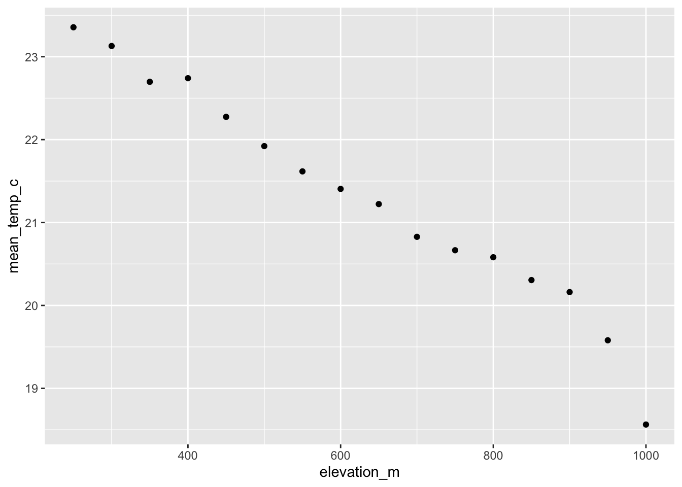

d. Temperature model

# model
temperature_model <- lm(
  mean_temp_c ~ elevation_m, # formula: response ~ predictor
  data = sonadora_sum # data frame
  )

Diagnostics

# diagnostics
par(mfrow = c(2, 2))
plot(temperature_model)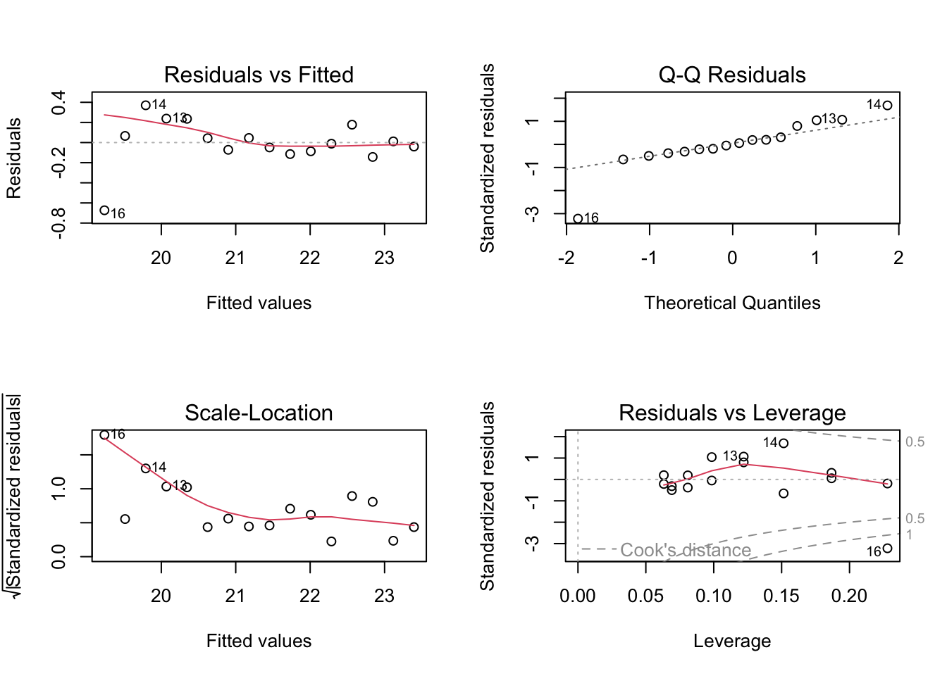

Model summary

summary(temperature_model)

Call:
lm(formula = mean_temp_c ~ elevation_m, data = sonadora_sum)

Residuals:
     Min       1Q   Median       3Q      Max 
-0.67288 -0.07577  0.00022  0.09393  0.37042 

Coefficients:
              Estimate Std. Error t value Pr(>|t|)    
(Intercept) 24.7807991  0.1719438  144.12  < 2e-16 ***
elevation_m -0.0055446  0.0002581  -21.48 4.08e-12 ***
---
Signif. codes:  0 '***' 0.001 '**' 0.01 '*' 0.05 '.' 0.1 ' ' 1

Residual standard error: 0.238 on 14 degrees of freedom
Multiple R-squared:  0.9706,    Adjusted R-squared:  0.9684 
F-statistic: 461.4 on 1 and 14 DF,  p-value: 4.075e-12

For each meter of elevation gain, you would expect a decrease in temperature equivalent to 0.01 ± 0.0003 (SE) °C.

Generating predictions

# model predictions
temperature_preds <- ggpredict(
  temperature_model,      # model object
  terms = "elevation_m"   # predictor (in quotation marks)
)

# calculate the temperature prediction at elevation = 900
ggpredict(
  temperature_model,           # model object
  terms = "elevation_m[900]"   # predictor (in quotation marks) and predictor value in brackets
)

# Predicted values of mean_temp_c

elevation_m | Predicted |       95% CI
--------------------------------------
        900 |     19.79 | 19.59, 19.99

At 900 m, the predicted temperature is 19.8 °C (95% CI: [19.6, 20.0]).

Visualizing model predictions

# base layer
ggplot(data = sonadora_sum, 
       aes(x = elevation_m,
           y = mean_temp_c)) +
  # first layer: temperature at each elevation
  geom_point() +
  # 95% CI ribbon
  # uses model prediction data frame
  geom_ribbon(data = temperature_preds,
              aes(x = x,
                  y = predicted,
                  ymin = conf.low,
                  ymax = conf.high),
              alpha = 0.2) +
  # model prediction line
  # uses model prediction data frame
  geom_line(data = temperature_preds,
              aes(x = x,
                  y = predicted)) +
  # axis labels
  labs(x = "Elevation (m)",
       y = "Mean temperature (\U00B0 C)") +
  theme_bw()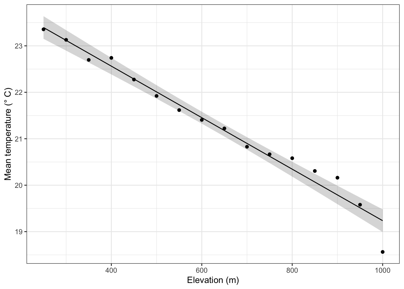

Creating a table with model coefficients, 95% confidence intervals, and more

tbl_regression(temperature_model,
               # make sure the y-intercept estimate is shown
               intercept = TRUE,
               # changing labels in "Characteristic" column
               label = list(`(Intercept)` = "Intercept",
                            elevation_m = "Elevation (m)")) |> 
  # changing header text
  modify_header(label = "**Variable**",
                estimate = "**Estimate**") |> 
  # turning table into a flextable (makes things easier to render to word or PDF)
  as_flex_table()

Variable	Estimate	95% CI	p-value
Intercept	25	24, 25	<0.001
Elevation (m)	-0.01	-0.01, 0.00	<0.001
Abbreviation: CI = Confidence Interval

END OF SONADORA EXAMPLE